Hookean elastic material

The Hookean elastic model describes linear elastic behavior of materials through a direct proportionality between stress and strain. Hooke’s law states:

\[\mathbf{S} = \mathbf{C}\,\boldsymbol{\varepsilon}\]

where:

• \(\mathbf{S}\) is the stress tensor (force per unit area).

• \(\mathbf{C}\) is the fourth-order elasticity tensor encoding material stiffness.

• \(\boldsymbol{\varepsilon}\) is the Green-Lagrange strain tensor defined as:

This relation holds as long as the deformation remains small, meaning the material stays near its rest configuration (:math:|boldsymbol{varepsilon}| ll 1). This small-strain assumption defines what is often referred to as the Hookean regime.

\[\boldsymbol{\varepsilon} = \frac{1}{2}(\mathbf{F}^T \mathbf{F} - \mathbf{I})\]

where \(\mathbf{F}\) is the deformation gradient and \(\mathbf{I}\) is the identity matrix, measures how much the material is deformed.

The Hookean model corresponds to a quadratic energy potential given by:

\begin{align} W(\mathbf{F}) = \frac{1}{2}\boldsymbol{\varepsilon}:\mathbf{C}\boldsymbol{\varepsilon} = \frac{1}{2}\boldsymbol{\varepsilon}:\mathbf{S} \end{align}

where “:” denotes the double inner product, or tensor contraction.

Its gradient is given as expected by:

\[\frac{\partial W}{\partial \varepsilon} = \mathbf{C}\boldsymbol{\varepsilon} = \mathbf{S},\]

meaning \(W(\mathbf{F})\) is the energy potential associated with the stresses \(\mathbf{S}\).

Small perturbations of identity

Let’s assume we are in the case of Hooke’s regime where \(\mathbf{F}\) is a small perturbation of the identity matrix, i.e., \(x^{t+1} = F x^t\) where \(\mathbf{F} = \mathbf{I} + \nabla \mathbf{u}\). In this case, we can approximate the strain tensor as:

\[\boldsymbol{\varepsilon} = \frac{1}{2}(\nabla \mathbf{u} + \nabla \mathbf{u}^T + \nabla \mathbf{u}^T\nabla \mathbf{u}) \approx \frac{1}{2}(\nabla \mathbf{u} + \nabla \mathbf{u}^T)\]

because nabla mathbf{u}^Tnabla mathbf{u} is negligible (\(\Vert\nabla u\Vert \ll 1\)) for small perturbations (linear model).

But, in Euclidean coordinates, and for an isotropic material, \(\mathbf{C}\) is defined as

\[C_{ijkl} = \lambda \delta_{ij}\delta_{kl} + \mu (\delta_{ik}\delta_{jl} + \delta_{il}\delta_{jk})\]

where \(\delta_{ij}\) is the Kronecker delta, and \(\lambda\) and \(\mu\) are the Lamé parameters.

We then have

\[\mathbf{C}\boldsymbol{\varepsilon} = \lambda \mathrm{tr}(\boldsymbol{\varepsilon})\mathbf{I} + 2\mu \boldsymbol{\varepsilon}\]

Substituting this into the energy potential, we obtain:

\[W(\mathbf{F}) = \frac{\lambda}{2} (\mathrm{tr}(\boldsymbol{\varepsilon}))^2 + \mu \boldsymbol{\varepsilon}:\boldsymbol{\varepsilon}\]

where \(\mathrm{tr}(\boldsymbol{\varepsilon})\) is the trace of the strain tensor, and \(\|\boldsymbol{\varepsilon}\|^2\) is the Frobenius norm of the strain tensor.

The first term of the equation simplifies to :

\[\frac{\lambda}{2}(\mathrm{tr}(\boldsymbol{\varepsilon}))^2 = \frac{\lambda}{2}(\varepsilon_{xx} + \varepsilon_{yy} + \varepsilon_{zz})^2\]

and the second term simplifies to:

\[\mu \boldsymbol{\varepsilon}:\boldsymbol{\varepsilon} = \mu (\varepsilon_{xx}^2 + \varepsilon_{yy}^2 + \varepsilon_{zz}^2 + 2\varepsilon_{xy}^2 + 2\varepsilon_{xz}^2 + 2\varepsilon_{yz}^2)\]

This means that the energy potential is a quadratic function of the deformation gradient \(\nabla \mathbf{u}\), and can be expressed as:

\[W(\mathbf{F}) = \left(\mu + \frac{\lambda}{2}\right)(\varepsilon_{xx}^2 + \varepsilon_{yy}^2 + \varepsilon_{zz}^2) + \lambda (\varepsilon_{xx} \varepsilon_{yy} + \varepsilon_{xx} \varepsilon_{zz} + \varepsilon_{yy} \varepsilon_{zz}) + 2\mu (\varepsilon_{xy}^2 + \varepsilon_{xz}^2 + \varepsilon_{yz}^2)\]

where \(\varepsilon_{ij} = \frac{1}{2}(\partial_i u_j + \partial_j u_i)\).

Here,

• the terms \(\varepsilon_{ii}\) represent the energy contribution from normal (axial) strain along the coordinate axes,

• the mixed terms \(\varepsilon_{ii} \varepsilon_{jj}\) represent the coupling between normal strains along different axes, contributing to the energy associated with volumetric deformation,

• the terms \(\varepsilon_{ij}^2\) represent the energy contribution from shear strain in the \((i, j)\) plane, penalizing angular distortions between coordinate directions.

Examples of Hookean energy responses

The Hookean model predicts a quadratic energy response with respect to the strain tensor \(\boldsymbol{\varepsilon}\) for small deformations, as the energy potential is of the form:

\[W(\mathbf{F}) = \frac{1}{2} \boldsymbol{\varepsilon} : \mathbf{C} \boldsymbol{\varepsilon}\]

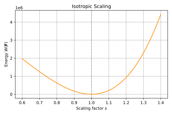
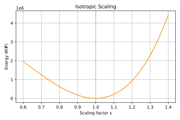
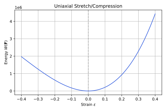
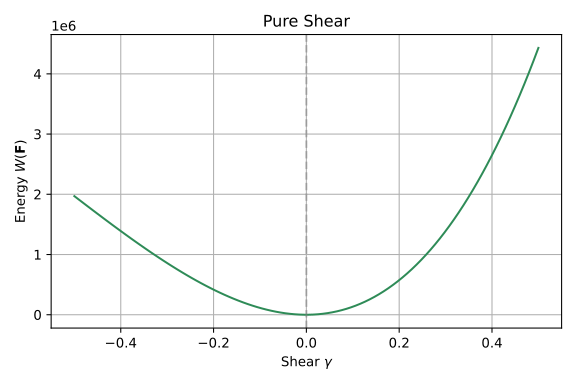
To validate this behavior in practice, we simulate several canonical deformations and plot the total elastic energy as a function of the deformation parameter.

We first start with the most simple deformation non-zero energy mode that can be expressed as an affine transformation, i.e., isotropic scaling.

The isotropic scaling deformation is defined as:

\[\begin{split}\mathbf{F} = s \cdot \mathbf{I} = \begin{bmatrix} s & 0 \\ 0 & s \end{bmatrix}\end{split}\]

where \(s\) is the scaling factor.

The strain tensor is then given by:

\[\boldsymbol{\varepsilon} = \frac{1}{2}(\mathbf{F}^T \mathbf{F} - \mathbf{I}) = \frac{1}{2}(s^2 - 1)\mathbf{I}.\]

As we can see, the components of the strain tensor are quadratic in the scaling factor \(s\). We then expect the elastic energy potential to be a quartic function of \(s\). We can then give an expression of the elastic energy potential as:

\[W(s) = \frac{\lambda + \mu}{2}(s^2 - 1)^2\]

where \(\lambda\) and \(\mu\) are the Lamé parameters.

This means that the energy potential is a quartic function of the scaling factor \(s\), and a quadratic function of the strain tensor \(\boldsymbol{\varepsilon}\).

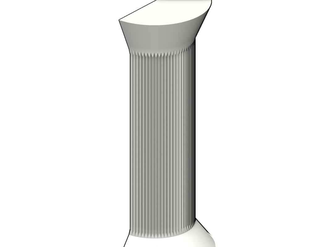
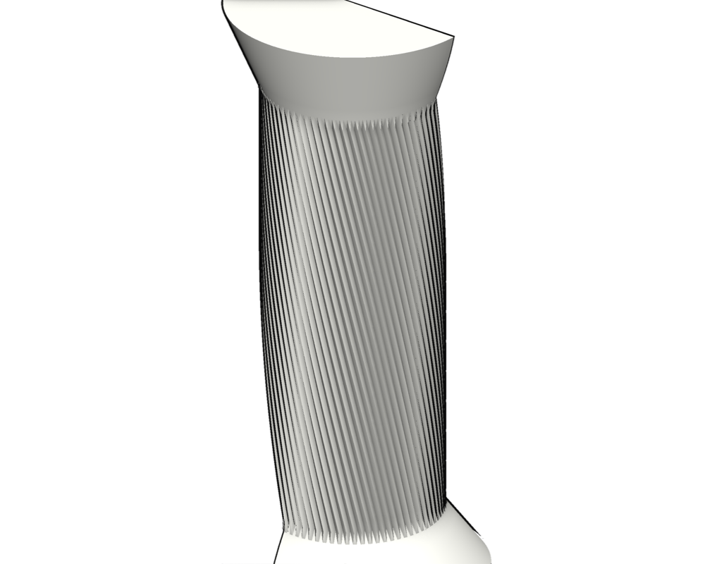
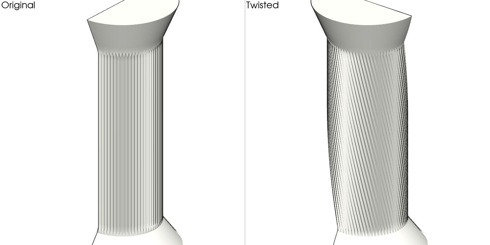
We also investigate 3D deformation modes that cannot be expressed as simple affine transformations, such as torsion and bending. These deformations are nonuniform but can still be analyzed under the Hookean regime by computing the Green–Lagrange strain pointwise.

We define the twisting deformation around the Z-axis with its deformation gradient as:

\[\begin{split}\mathbf{F}(x, y, z) = \begin{bmatrix} \cos\theta(z) & -\sin\theta(z) & -\frac{\theta_{\text{twist}}}{L}(x\sin\theta(z) + y\cos\theta(z)) \\ \sin\theta(z) & \cos\theta(z) & \frac{\theta_{\text{twist}}}{L}(x\cos\theta(z) - y\sin\theta(z)) \\ 0 & 0 & 1 \end{bmatrix}\end{split}\]

where \(\theta(z) = \frac{z}{L}\theta_{\text{twist}}\) is the angle of twist at position \(z\) along the column’s axis,

\(L\) is the length of the column, and \(\theta_{\text{twist}}\) is the maximum twist angle (in radians), corresponding

to the twist angle at the top of the column (\(z = L\)).

This deformation gradient is given pointwise, as the deformation is nonuniform.

Let’s consider a column of length \(L\):

that is twisted around the Z-axis with a maximum twist angle of \(\theta_{\text{twist}} = \pi\) radians:

The strain tensor is then given by:

\[\boldsymbol{\varepsilon} = \frac{1}{2}(\mathbf{F}^T \mathbf{F} - \mathbf{I}) = \frac{\theta_{\text{twist}}}{L} \left(x^2+y^2\right) + 1.\]

Here, the deformation being nonuniform, the strain tensor is also given pointwise. We see that it is quadratic in the parameter \(\theta_{\text{twist}}\), we then expect the elastic energy potential to be a quartic function of \(\theta_{\text{twist}}\).

We can then give a pointwise expression of the elastic energy potential as:

\[W(\theta_{\text{twist}}, x, y) = \frac{\lambda}{8}\frac{\theta_{\text{twist}}^4}{L^4}(x^2 + y^2)^2 + \frac{\mu}{4}\frac{\theta_{\text{twist}}^2}{L^2}\left(2x^2 + 2y^2 + \frac{\theta_{\text{twist}}^2}{L^2}(x^2 + y^2)^2\right)\]

As expected, the energy potential is a quartic function of the twist angle \(\theta_{\text{twist}}\), and a quadratic function of the strain tensor \(\boldsymbol{\varepsilon}\).

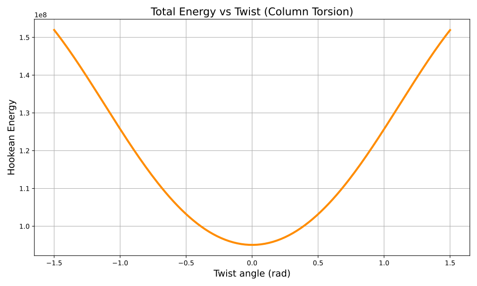
If we compute the sum of the elastic energy potential over the whole column with finite elements, we obtain the total elastic energy profile:

that looks quadratic.

Description of standard deformations and their energies

Isotropic scaling

• Description: Uniform expansion or compression in all directions

• Deformation gradient:

  \[\begin{split}\mathbf{F} = s \cdot \mathbf{I} = \begin{bmatrix} s & 0 \\ 0 & s \end{bmatrix}\end{split}\]

• Elastic energy potential:

  \[W(s) = \frac{\lambda + \mu}{2}(s^2 - 1)^2\]

  

Uniaxial stretch / compression

• Description: Stretch or compress along the X axis

• Deformation gradient:

  \[\begin{split}\mathbf{F} = \begin{bmatrix} 1 + \varepsilon & 0 \\ 0 & 1 \end{bmatrix}\end{split}\]

• Elastic energy potential:

  \[W(\varepsilon) = \frac{\lambda + 2\mu}{8}(\varepsilon^2 - 1)^2\]

  

Pure shear

• Description: Shear in the X direction along the Y axis

• Deformation gradient:

  \[\begin{split}\mathbf{F} = \begin{bmatrix} 1 & \gamma \\ 0 & 1 \end{bmatrix}\end{split}\]

• Elastic energy potential:

  \[W(\gamma) = \frac{\lambda + 2\mu}{8}\gamma^4 + \frac{\mu}{2}\gamma^2\]

  

Bending (3D)

• Description: Beam bent along XZ plane (Euler-Bernoulli model for a cantilever beam)

• Deformation gradient:

  \[\begin{split}\mathbf{F}(x, z) = \begin{bmatrix} 1 - z\theta_x'\cos\theta_x & 0 & -\sin\theta_x \\ 0 & 1 & 0 \\ w'(x) - z\theta_x'\sin\theta_x & 0 & \cos\theta_x \end{bmatrix}\end{split}\]
  where \(w(x) = \frac{F}{6EI}x^2(3L - x)\) is the deflection of the beam at position \(x\),

  \(F\) is the force applied at the end of the beam,

  \(\theta_x = \arctan w'(x)\) is the angle of rotation of the beam at position \(x\),

  and \(\theta_x' = \frac{d\theta_x}{dx}\) is the derivative of the angle of rotation with respect to \(x\).

• Elastic energy potential:

  \[\begin{split}W(F, x, z) = \frac{\lambda}{8}\left(z^2\theta_x'^2 + w'(x)^2 - 2z\theta_x'(\cos\theta_x + w'(x)\sin\theta_x)\right) \\ + \frac{\mu}{4}\left((z^2\theta_x'^2 + w'(x)^2 - 2z\theta_x'(\cos\theta_x + w'(x)\sin\theta_x))^2 + 2(w'(x)\cos\theta_x - \sin\theta_x)^2\right)\end{split}\]

Torsion (3D)

• Description: Twisting column around the Z axis

  

• Deformation gradient:

  \[\begin{split}\mathbf{F}(x, y, z) = \begin{bmatrix} \cos\theta(z) & -\sin\theta(z) & -\frac{\theta_{\text{twist}}}{L}(x\sin\theta(z) + y\cos\theta(z)) \\ \sin\theta(z) & \cos\theta(z) & \frac{\theta_{\text{twist}}}{L}(x\cos\theta(z) - y\sin\theta(z)) \\ 0 & 0 & 1 \end{bmatrix}\end{split}\]
  where \(\theta(z) = \frac{z}{L}\theta_{\text{twist}}\) is the angle of twist at position \(z\) along the column’s axis,

  \(L\) is the length of the column,

  and \(\theta_{\text{twist}}\) is the maximum twist angle (in radians), corresponding to the twist angle at the top of the column (\(z = L\))

• Elastic energy potential:

  \[\begin{split}W(\theta_{\text{twist}}, x, y) = \frac{\lambda}{8}\frac{\theta_{\text{twist}}^4}{L^4}(x^2 + y^2)^2 \\ + \frac{\mu}{4}\frac{\theta_{\text{twist}}^2}{L^2}\left(2x^2 + 2y^2 + \frac{\theta_{\text{twist}}^2}{L^2}(x^2 + y^2)^2\right)\end{split}\]

Rigid rotations and rigid translations

Let’s now see what happens in the other cases of Hooke’s regime, i.e., when the deformation is a rigid rotation or a rigid translation.

For a rigid translation, \(x^{t+1} = x^t + \mathbf{u}\). In this case, the deformation gradient is simply the identity matrix, and the strain tensor is zero.

For a rigid rotation, \(x^{t+1} = R x^t\) where \(R\) is a rotation matrix. In this case, the deformation gradient is \(R\), and the strain tensor is again zero.

These deformations are called zero-energy modes because they do not contribute to the energy potential.

Zero Energy Modes

Rigid translations and rotations do not produce strain and therefore store no elastic energy.

They form the set of deformation modes that lie entirely within the nullspace of the elastic energy. A well-defined Hookean model must be invariant under these transformations.