How to compute local geometric moments

We use the point_moments() method to compute local averages and covariance matrices. This is useful for estimating point normals and curvatures.

First, we create a simple point cloud in 2D:

import torch
from matplotlib import pyplot as plt

import skshapes as sks

n_points, dim = 3, 2
shape = sks.PolyData(torch.rand(n_points, dim))
print(shape)

skshapes.PolyData (0x7fa88f604e50 on cpu, float32), a 2D point cloud with:
- 3 points
- center (0.431, 0.124), radius 0.238
- bounds x=(0.222, 0.601), y=(0.029, 0.238),

The method point_neighborhoods() associates to each point \(x_i\) in the shape a weight distribution \(\nu_i(x)\) over the ambient space. Typically, this corresponds to a normalized Gaussian window at scale \(\sigma\). If \(\mu(x)\) denotes the uniform distribution on the support of the shape, then:

\[\nu_i(x) \propto \exp\left(-\frac{||x-x_i||^2}{2\sigma^2}\right) \mu(x)\]

The method point_moments() takes as input the same arguments, and returns a skshapes.features.Moments object that computes the moments of order 0, 1 and 2 of these distributions.

moments = shape.point_moments(scale=0.5)

The total mass \(m_i\) of \(\nu_i\) is an estimate of the local point density:

print(moments.masses)

tensor([2.9560, 2.4417, 2.6095])

The local mean \(\overline{x}_i = \mathbb{E}_{x\sim \nu_i}[x]\) is a point in the vicinity of \(x_i\):

print(moments.means)

tensor([[0.4366, 0.1215],
        [0.4045, 0.1391],
        [0.4529, 0.1125]])

The local covariance matrix \(\Sigma_i = \mathbb{E}_{x\sim \nu_i}[(x-\overline{x}_i)(x-\overline{x}_i)^{\intercal}]\) is symmetric and positive semi-definite:

print(moments.covariances)

tensor([[[ 0.0242, -0.0133],
         [-0.0133,  0.0073]],

        [[ 0.0255, -0.0140],
         [-0.0140,  0.0077]],

        [[ 0.0230, -0.0126],
         [-0.0126,  0.0070]]])

Its eigenvalues are non-negative and typically of order \(\sigma^2\):

L = moments.covariance_eigenvalues
print(L)

tensor([[2.3372e-06, 3.1545e-02],
        [4.1747e-06, 3.3108e-02],
        [4.6184e-06, 2.9921e-02]])

Its eigenvectors are orthogonal and represent the principal directions of the local distribution of points:

Q = moments.covariance_eigenvectors
print(Q)

tensor([[[-0.4819, -0.8762],
         [-0.8762,  0.4819]],

        [[-0.4807, -0.8769],
         [-0.8769,  0.4807]],

        [[-0.4826, -0.8759],
         [-0.8759,  0.4826]]])

The eigenvectors are stored column-wise, and sorted by increasing eigenvalue:

LQt = L.view(n_points, dim, 1) * Q.transpose(1, 2)
QLQt = Q @ LQt

print(f"Reconstruction error: {(QLQt - moments.covariances).abs().max():.2e}")

Reconstruction error: 5.59e-09

Note

These attributes are computed when required, and cached in memory.

On a 2D curve

Going further, let’s consider a sampled curve in 2D:

shape = sks.doc.wiggly_curve(n_points=32, dim=2)
print(shape)

skshapes.PolyData (0x7fa890d6fe90 on cpu, float32), a 2D point cloud with:
- 32 points
- center (-0.078, 0.224), radius 1.283
- bounds x=(-1.076, 1.196), y=(-0.923, 1.098),

Intuitively, computing local moments \(m_i\) of order 0, \(\overline{x}_i\) of order 1 and \(\Sigma_i\) of order 2 is equivalent to fitting a Gaussian distribution to each local neighborhood \(\nu_i\). In dimension \(D=2\) or \(D=3\), if \(\lambda_{\mathbb{R}^D}\) denotes the Lebesgue measure on the ambient space (i.e. the area or the volume), then:

\[\begin{split}\text{d}\nu_i(x) ~&\simeq~ m_i\,\text{d}\mathcal{N}(\overline{x}_i, \Sigma_i)(x) \\ &= ~\frac{m_i}{(2\pi\sigma^2)^{D/2} } \, \exp\left[-\tfrac{1}{2}(x-\overline{x}_i)^{\intercal}\Sigma_i^{-1}(x-\overline{x}_i)\right]\, \text{d}\lambda_{\mathbb{R}^D}(x)~\end{split}\]

We visualize these descriptors by drawing ellipses centered at \(\overline{x}_i\), colored by the local densities \(m_i\) and oriented in \(\mathbb{R}^2\) or \(\mathbb{R}^3\) with axes that are aligned with the eigenvectors of \(\Sigma_i\) and whose lengths are proportional to the square root of its eigenvalues:

plt.figure(figsize=(12, 10))

for i, sigma in enumerate([0.1, 0.2, 0.5, 1.0]):
    moments = shape.point_moments(scale=sigma)

    # Plot the ellipses
    ax = plt.subplot(2, 2, i + 1)
    ax.set_title(f"Moments at scale = {sigma:.1f}")
    sks.doc.display_covariances(shape.points, moments)

plt.tight_layout()

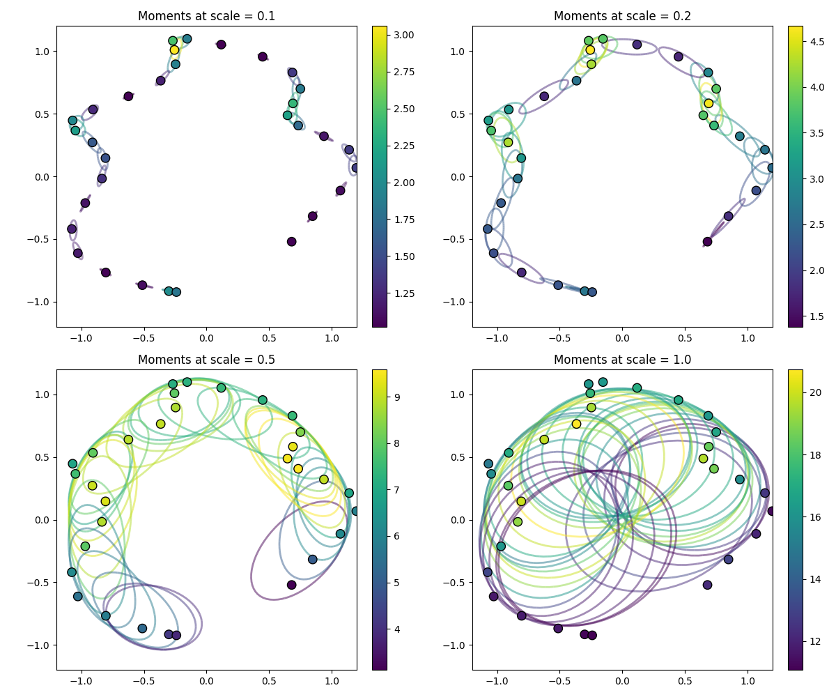
As evidenced here, point_moments() describes the local shape context at scale \(\sigma\). We use it to compute point normals and curvatures that are robust to noise and sampling artifacts.

On a 3D surface

We can perform the same analysis on a 3D surface:

import pyvista as pv

shape = (
    sks.PolyData(pv.examples.download_bunny())
    .resample(n_points=5000)
    .normalize()
)
print(shape)

skshapes.PolyData (0x7fa890910850 on cpu, float32), a 3D triangle mesh with:
- 5,000 points, 14,952 edges, 9,949 triangles
- center (-0.000, 0.000, 0.000), radius 1.000
- bounds x=(-0.581, 0.767), y=(-0.534, 0.807), z=(-0.597, 0.453)

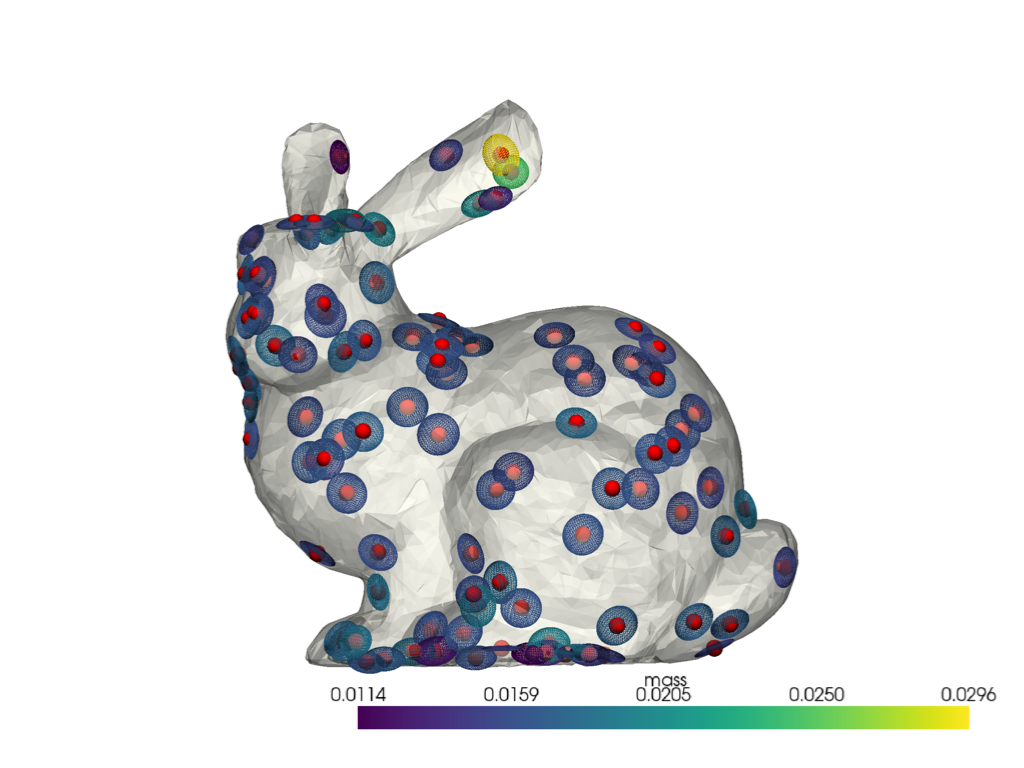
As expected, the point moments of order 1 and 2 now refer to 3D vectors and matrices:

moments = shape.point_moments(scale=0.05)
print("moments.masses:     ", moments.masses.shape)
print("moments.means:      ", moments.means.shape)
print("moments.covariances:", moments.covariances.shape)

moments.masses:      torch.Size([5000])
moments.means:       torch.Size([5000, 3])
moments.covariances: torch.Size([5000, 3, 3])

We visualize the ellipsoids on a subset of our full point cloud:

landmark_indices = list(range(0, shape.n_points, 50))

pl = pv.Plotter()
sks.doc.display(plotter=pl, shape=shape, opacity=0.5)
sks.doc.display_covariances(
    shape.points, moments, landmark_indices=landmark_indices, plotter=pl
)
pl.show()

Static Scene

Interactive Scene

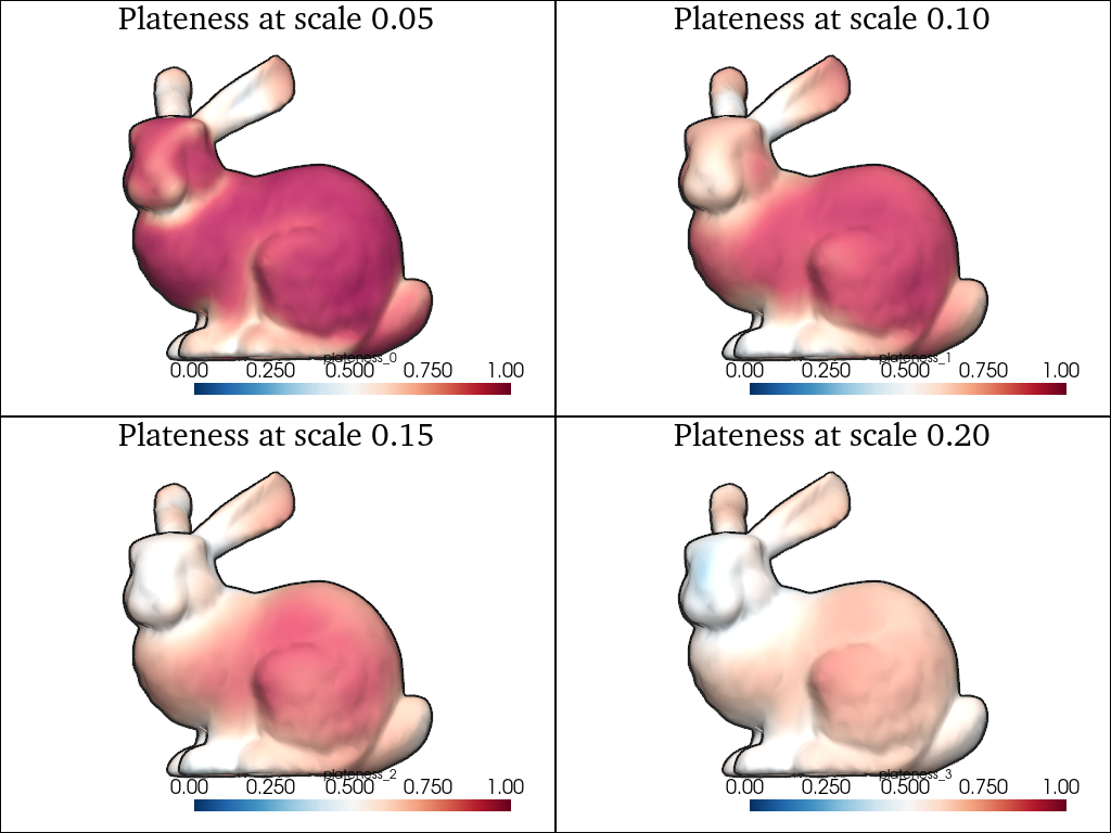
Using the covariance eigenvalues \(\lambda_1 \leqslant \lambda_2 \leqslant \lambda_3\), we can compute simple shape descriptors such as the plateness which is equal to 0 if the local ellipsoid is a sphere and 1 if it is a 2D disk:

\[\text{plateness} = 1 - \frac{\lambda_1}{\sqrt{\lambda_2\lambda_3}}~.\]

scales = [0.05, 0.1, 0.15, 0.2]

pl = pv.Plotter(shape=(2, 2))
for i, scale in enumerate(scales):
    moments = shape.point_moments(scale=scale)
    eigs = moments.covariance_eigenvalues
    shape.point_data[f"plateness_{i}"] = (
        1 - eigs[:, 0] / (eigs[:, 1] * eigs[:, 2]).sqrt()
    )

    pl.subplot(i // 2, i % 2)
    sks.doc.display(
        plotter=pl,
        shape=shape,
        scalars=f"plateness_{i}",
        scalar_bar=True,
        smooth=1,
        clim=(0, 1),
        title=f"Plateness at scale {scale:.2f}",
    )
pl.show()

Static Scene

Interactive Scene

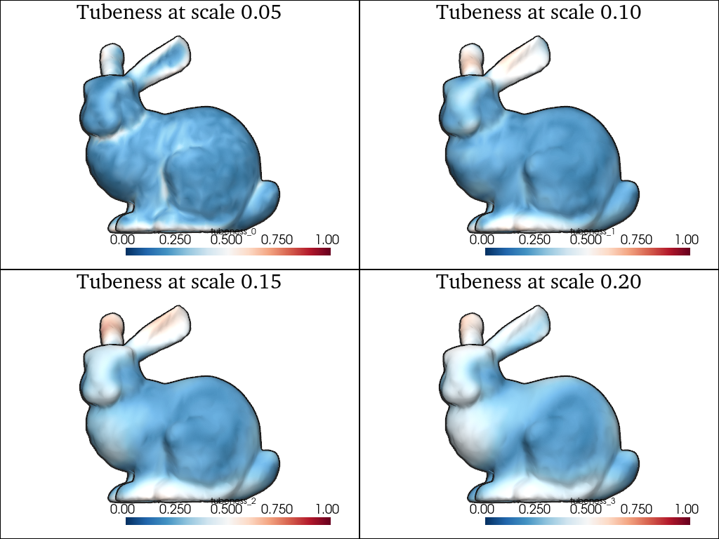
Likewise, we can compute the tubeness, which is equal to 0 if the local ellipsoid is a sphere or a disk, and 1 if it is a 1D segment:

\[\text{tubeness} = 1 - \frac{\lambda_2}{\lambda_3}~.\]

pl = pv.Plotter(shape=(2, 2))
for i, scale in enumerate(scales):
    moments = shape.point_moments(scale=scale)
    eigs = moments.covariance_eigenvalues
    shape.point_data[f"tubeness_{i}"] = 1 - (eigs[:, 1] / eigs[:, 2])

    pl.subplot(i // 2, i % 2)
    sks.doc.display(
        plotter=pl,
        shape=shape,
        scalars=f"tubeness_{i}",
        scalar_bar=True,
        smooth=1,
        clim=(0, 1),
        title=f"Tubeness at scale {scale:.2f}",
    )
pl.show()

Static Scene

Interactive Scene