How to compute local point normals

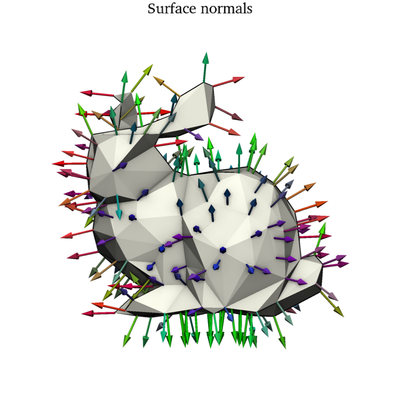
We use the point_normals() method to compute normal vectors at each vertex of a triangle mesh. This is useful for estimating the curvature of the surface.

First, we load the Stanford bunny as a triangle mesh.

import pyvista as pv

import skshapes as sks

mesh = sks.PolyData(pv.examples.download_bunny())

# To improve the readability of the figures below, we resample the mesh to have
# a fixed number of points and normalize it to fit in the unit sphere.
mesh = mesh.resample(n_points=200).normalize()

Then, we compute the point normals.

normals = mesh.point_normals()

sks.doc.display(
    title="Surface normals",
    shape=mesh,
    vectors=-0.2 * normals,
    vectors_color=normals.abs(),
)

Static Scene

Interactive Scene

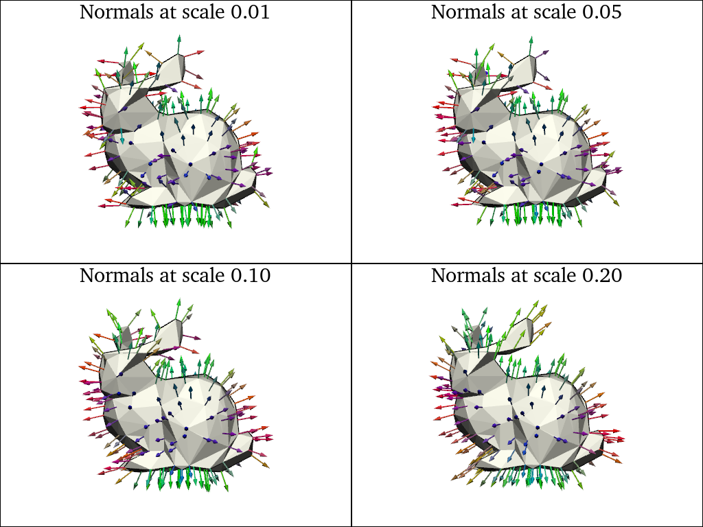
Then, we compute the point normals.

pl = pv.Plotter(shape=(2, 2))

for i, scale in enumerate([0.01, 0.05, 0.1, 0.2]):

    normals = mesh.point_normals(scale=scale)

    pl.subplot(i // 2, i % 2)
    sks.doc.display(
        title=f"Normals at scale {scale:.2f}",
        plotter=pl,
        shape=mesh,
        vectors=-0.2 * normals,
        vectors_color=normals.abs(),
    )

pl.show()

Static Scene

Interactive Scene

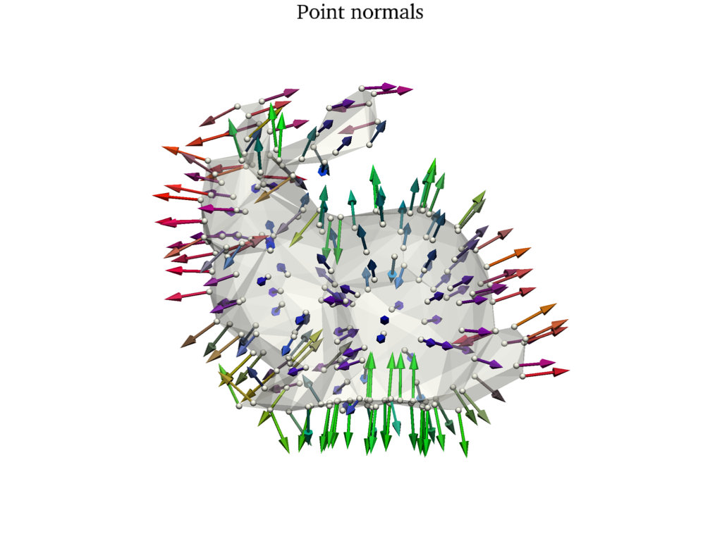
Then, we compute the point normals.

points = mesh.to_point_cloud()
normals = points.point_normals(scale=0.1)

pl = pv.Plotter()
sks.doc.display(plotter=pl, shape=mesh, opacity=0.3)
sks.doc.display(
    plotter=pl,
    title="Point normals",
    shape=points,
    point_size=20,
    vectors=0.2 * normals,
    vectors_color=normals.abs(),
)
pl.show()

Static Scene

Interactive Scene