Multiscaling and signal propagation

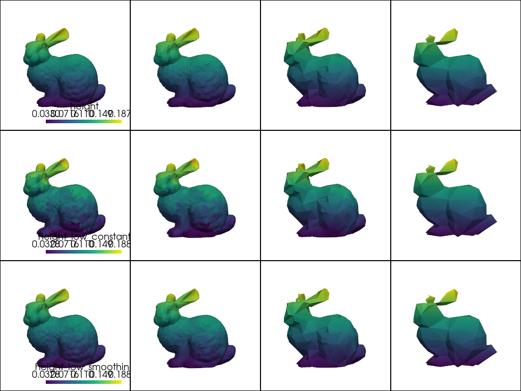
We propagate a signal across the different shapes of a multiscale representation, using rules that are specified by a FineToCoarsePolicy and a CoarseToFinePolicy.

First, we load the Stanford bunny as a triangle mesh and sub-sample it using 10%, 1% and 0.5% of the original point count.

import pyvista as pv

import skshapes as sks

bunny = sks.PolyData(pv.examples.download_bunny())
ratios = [1, 0.1, 0.01, 0.001]
multiscale_bunny = sks.Multiscale(shape=bunny, ratios=ratios)

Then, we define a signal on the original, high resolution surface mesh.

# Extract the 2nd coordinate "y" of each point "xyz"
signal = multiscale_bunny.at(ratio=1).points[:, 1]

# Use it as a "height" signal
multiscale_bunny.at(ratio=1).point_data["height"] = signal

We use the propagate() method to transfer the signal from our high resolution mesh to the coarser scales.

Note

Accessing the multiscale representation at ratio=1 always returns the finest shape.

multiscale_bunny.propagate(
    signal_name="height",
    from_ratio=1,
    fine_to_coarse_policy=sks.FineToCoarsePolicy(reduce="mean"),
)

pl = pv.Plotter(shape=(2, 2))
for i, ratio in enumerate(ratios):
    pl.subplot(i // 2, i % 2)
    sks.doc.display(
        plotter=pl, shape=multiscale_bunny.at(ratio=ratio), scalars="height"
    )
pl.show()

Static Scene

Interactive Scene

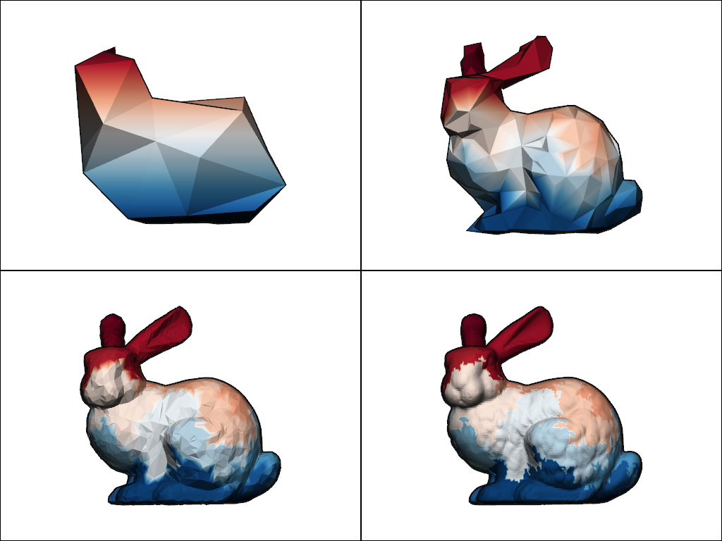
Conversely, let us propagate a signal from the coarser resolutions to the finer levels of detail.

Note

Accessing the multiscale representation at ratio=0 always returns the coarsest shape.

signal_coarse = multiscale_bunny.at(ratio=0).points[:, 1]
multiscale_bunny.at(ratio=0).point_data["signal"] = signal_coarse

# propagate the signal from the lower resolutions to the higher resolution
multiscale_bunny.propagate(
    signal_name="signal",
    from_ratio=0,
    coarse_to_fine_policy=sks.CoarseToFinePolicy(smoothing="constant"),
)

pl = pv.Plotter(shape=(2, 2))
for i, ratio in enumerate(reversed(ratios)):
    pl.subplot(i // 2, i % 2)
    sks.doc.display(
        plotter=pl, shape=multiscale_bunny.at(ratio=ratio), scalars="signal"
    )
pl.show()

Static Scene

Interactive Scene

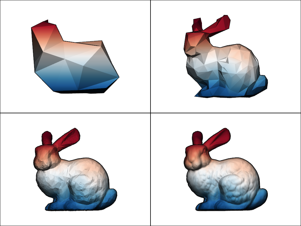
The "constant" policy results in sharp transitions between regions of the surface that were collapsed to the same coarse point. To mitigate this issue, we can use a "mesh_convolution" CoarseToFinePolicy that interleaves smoothing steps between the jumps from coarse to fine scales.

multiscale_bunny.propagate(
    signal_name="signal",
    from_ratio=0,
    coarse_to_fine_policy=sks.CoarseToFinePolicy(
        smoothing="mesh_convolution",
        n_smoothing_steps=2,
    ),
)

pl = pv.Plotter(shape=(2, 2))
for i, ratio in enumerate(reversed(ratios)):
    pl.subplot(i // 2, i % 2)
    sks.doc.display(
        plotter=pl, shape=multiscale_bunny.at(ratio=ratio), scalars="signal"
    )
pl.show()

Static Scene

Interactive Scene