Note

Go to the end to download the full example code

Elastic metric and multiscale strategy¶

This examples is an implementation of the paper “Geometric Modeling in Shape Space” by Kilian, Mitra and Pottmann. More precisely, we implement the algorithm for the Boundary Value Problem, which is a registration between two shapes.

The framework proposed in the paper allows to find a deformation between two shapes that minimizes an elastic metric. Optimizing directly the deformation in full resolution and with a large number of steps usually leads to bad local minima. To avoid this, the authors propose a multiscale strategy, where the optimization is first performed in a coarse resolution and with a small number of steps. Then, refinement can be done by increasing the resolution (space refinement) or the number of steps (time refinement).

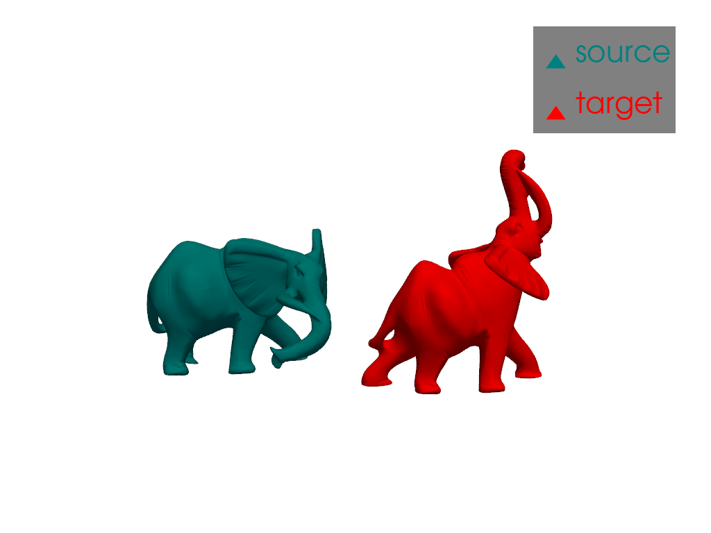
In this example, we provide an implementation of the “Boundary Value Problem” algorithm describe in section 3, using the as isometric as possible metric, defined at the end of section 2. The algorithm is applied to the registration of two elephant poses.

Load the data¶

import pyvista as pv
import torch

import skshapes as sks

source_color = "teal"
target_color = "red"

source = sks.PolyData("../data/elephants/pose_B.obj")
target = sks.PolyData("../data/elephants/pose_A.obj")

# Make sure that underlying simplicial complex are the same
triangles = source.triangles
target.triangles = source.triangles

plotter = pv.Plotter()
plotter.add_mesh(source.to_pyvista(), color=source_color, label="source")
plotter.add_mesh(target.to_pyvista().translate([250, 0, 0]), color=target_color, label="target")
plotter.camera_position = [
    (107.13691493781944, -436.8511227598446, 929.44474582162),
    (138.38692092895508, -5.646553039550781, 2.4097938537597656),
    (-0.07742352421458944, 0.9049853883599757, 0.41833843327279513)
    ]
plotter.add_legend()
plotter.show()

Static Scene

Interactive Scene

Define function for Space refinement¶

Space refinement is the process of refining the path by projecting the points of the fine mesh on the coarse mesh.

Each fine mesh can be projected to a coarse mesh,resulting in a system of coordinates. The coordinates consist of (for each point of the fine mesh):

the id of the closer triangle in the coarse mesh
the barycentric coordinates of the point in the triangle (2 coordinates)
the orthogonal coordinate of the point with respect to the triangle normal

With this system of coordinate, a coarse mesh with the same triangles as the one used to define the coordinates can be refined to a finer mesh. It is done by positioning points in the triangle of the coarse mesh and adding the orthogonal coordinate to the position.

The space refinement process consists in:

projecting the fine source and target on the coarse source and target
refining the coarse sequence of poses to a fine sequence of poses for both systems of coordinates
defining the fine sequence as a linear combination of the two refined sequences

This step lead to a fine sequence of poses in at the fine resolution. The registration model can then be refitted to minimize the energy.

This process is described in the section 3, paragraph “The Boundary Value Problem”.

from trimesh import Trimesh
from trimesh.proximity import closest_point
from trimesh.triangles import barycentric_to_points, points_to_barycentric


@torch.no_grad
def compute_coordinates(
    fine: sks.PolyData,
    coarse: sks.PolyData
    ) -> tuple[
        sks.Int1dTensor,
        sks.Float2dTensor,
        sks.Float1dTensor
    ]:
    """Compute coordinates of the fine points in the coarse mesh.

    We follow the approach of "Geometric Modeling in Shape Space", the coordinates
    are the id of the triangle, the 2D barycentric coordinates in the triangle
    and the distance between the point and his projection in the normal direction.

    Parameters
    ----------
    fine
        The PolyData object of the fine mesh
    coarse
        The PolyData object of the coarse mesh

    Returns
    -------
    tuple
        The id of the triangle, the barycentric coordinates and the orthogonal coordinate
        for each fine point.
    """

    if not fine.n_points >= coarse.n_points:
        msg = f"The fine mesh should have more points than the coarse mesh, got {fine.n_points} and {coarse.n_points}"
        raise ValueError(msg)

    faces = coarse.triangles.numpy()
    vertices = coarse.points.numpy()

    fine_points = fine.points.numpy()

    mesh = Trimesh(vertices=vertices, faces=faces)

    closest, distance, triangle_id = closest_point(mesh=mesh, points=fine_points)

    triangle_id = torch.tensor(triangle_id, dtype=sks.int_dtype)
    closest = torch.tensor(closest, dtype=sks.float_dtype)

    assert triangle_id.shape == (fine.n_points,)
    assert closest.shape == fine.points.shape

    t = coarse.points[coarse.triangles[triangle_id]]

    barycentric = points_to_barycentric(points=closest, triangles=t)

    # descr = (triangle_id, barycentric, product with normal)

    normals = coarse.triangle_normals / coarse.triangle_normals.norm(dim=-1, keepdim=True)

    # p - p' = fine_points - closest
    a = fine.points - closest

    Ns = normals[triangle_id]

    assert a.shape == Ns.shape

    # scalar product
    orthogonal_coordinate = (a * Ns).sum(dim=-1)

    return triangle_id, barycentric, orthogonal_coordinate



@torch.no_grad
def refine(
    coarse_mesh,
    coord_barycentric,
    triangle_id,
    orthogonal_coordinate
):
    """Given a system of coordinates, refine the points in the origin mesh.

    Parameters
    ----------
    coarse_mesh
        The mesh to refine
    coord_barycentric
        The barycentric coordinates of the fine points
    triangle_id
        The id of the triangle in the coarse mesh for each fine point
    orthogonal_coordinate
        The orthogonal coordinate of the fine points with respect to the triangle normal

    Returns
    -------
    sks.Points
        The fine points
    """

    Ns = coarse_mesh.triangle_normals[triangle_id] / coarse_mesh.triangle_normals[triangle_id].norm(dim=-1, keepdim=True)

    # Get the triangle
    t = coarse_mesh.points[coarse_mesh.triangles[triangle_id]]

    # Compute the orthogonal coordinate
    orthogonal = orthogonal_coordinate.repeat(3, 1).T * Ns

    # Compute the projection on the triangles
    projections = barycentric_to_points(barycentric=coord_barycentric, triangles=t)
    projections = torch.tensor(projections, dtype=sks.float_dtype)

    return projections + orthogonal

def space_refinement(
        coarse_source: sks.PolyData,
        coarse_target: sks.PolyData,
        fine_source: sks.PolyData,
        fine_target: sks.PolyData,
        coarse_model: sks.BaseModel,
        coarse_parameter: torch.Tensor,
        loss: sks.BaseLoss,
        regularization_weight: float,
        optimizer: sks.BaseOptimizer=lbfgs,
        n_iter: int=4,
        gpu: bool=True,
        verbose: bool=False
        ) -> tuple[torch.Tensor, sks.BaseModel]:
    """Refine the path following the space refinement strategy.

    We start by refining the path from coarse to high resolution and then
    optimize it with respect to the Riemannian metric (this optimization can
    be disabled by setting n_iter=0)

    The output is the parameter in the fine scale and the new model that can
    be used later on for registration.

    Parameters
    ----------
    coarse_source
        The source shape in coarse resolution.
    coarse_target
        The target shape in coarse resolution.
    fine_source
        The source shape in fine resolution.
    fine_target
        The target shape in fine resolution.
    coarse_model
        The model in coarse resolution.
    coarse_parameter
        The parameter in coarse resolution.
    loss
        The loss object for the registration.
    regularization_weight
        The regularization weight.
    optimizer
        The optimizer.
    n_iter
        The number of iterations.
    gpu
        Whether to use the GPU (if available).
    verbose
        Whether to print information during the process.

    Returns
    -------
        The parameter and the model in fine resolution.
    """


    # Compute the path at coarse level
    coarse_path = coarse_model.morph(shape=coarse_source, parameter=coarse_parameter, return_path=True).path

    # Copy the model
    fine_model = coarse_model.copy()

    if coarse_model.endpoints is not None:
        fine_model.endpoints = fine_target.points

    if verbose:
        print("Projecting the fine meshes on the coarse meshes...")

    # Compute the coordinates of the fine points in the coarse meshes
    triangle_id_source, barycentric_coord_source, orthogonal_coordinate_source = compute_coordinates(fine_source, coarse_source)
    triangle_id_target, barycentric_coord_target, orthogonal_coordinate_target = compute_coordinates(fine_target, coarse_target)


    fine_parameter = fine_model.inital_parameter(shape=fine_source)
    print(fine_parameter.shape)
    # fine_parameter = torch.zeros(size=(fine_source.n_points, fine_model.n_free_steps, 3), dtype=sks.float_dtype)

    new_points = torch.zeros_like(fine_source.points, dtype=sks.float_dtype)
    previous_points = torch.zeros_like(fine_source.points, dtype=sks.float_dtype)

    if verbose:
        print("Refining the path from coarse to fine...")

    for i, p in enumerate(coarse_path):

        previous_points = new_points

        if i == 0:
            # Force the first point to be the source
            new_points = fine_source.points

        if i == len(coarse_path) - 1 and coarse_model.endpoints is not None:
            # Force the last point to be the target
            print("ok")
            new_points = fine_target.points
            coarse_model.endpoints = fine_target.points

        else:
            newpoints_source = refine(
                coarse_mesh=p,
                coord_barycentric=barycentric_coord_source,
                triangle_id=triangle_id_source,
                orthogonal_coordinate=orthogonal_coordinate_source
                )

            newpoints_target = refine(
                coarse_mesh=p,
                coord_barycentric=barycentric_coord_target,
                triangle_id=triangle_id_target,
                orthogonal_coordinate=orthogonal_coordinate_target
                )

            new_points = ((i+1) / len(coarse_path)) * newpoints_source + (1 - (i+1) / len(coarse_path)) * newpoints_target

            fine_parameter[:, i-1, :] = new_points - previous_points

    if verbose:
        print("Optimizing the fine path wrt the metric...")

    registration = sks.Registration(
        model=fine_model,
        loss=loss,
        optimizer=optimizer,
        n_iter=n_iter,
        regularization_weight=regularization_weight,
        verbose=verbose,
        gpu=gpu,
    )

    registration.model = fine_model
    registration.fit(source=fine_source, target=fine_target, initial_parameter=fine_parameter)

    return registration.parameter_, fine_model

Multiscale representation¶

Back to our example, we first decimate the source and target shapes to a coarseer resolution. The decimation is done in parallel for both shapes to keep the correspondence between the points.

n_points_coarse = 650

# Parallel decimation of source and target
# the same decimation module is used for creating the multiscale representation
# of the source and target
decimation_module = sks.Decimation(n_points=650)
decimation_module.fit(source)
n_points = [n_points_coarse]

multisource = sks.Multiscale(source, n_points=n_points, decimation_module=decimation_module)
multitarget = sks.Multiscale(target, n_points=n_points, decimation_module=decimation_module)

coarse_source = multisource.at(n_points=n_points_coarse)
coarse_target = multitarget.at(n_points=n_points_coarse)
fine_source = multisource.at(n_points=source.n_points)
fine_target = multitarget.at(n_points=target.n_points)

# Plot the coarse source and target
plotter = pv.Plotter()
plotter.add_mesh(coarse_source.to_pyvista(), color=source_color, label="coarse source")
plotter.add_mesh(coarse_target.to_pyvista().translate([250, 0, 0]), color=target_color, label="coarse target")
plotter.camera_position = [
    (107.13691493781944, -436.8511227598446, 929.44474582162),
    (138.38692092895508, -5.646553039550781, 2.4097938537597656),
    (-0.07742352421458944, 0.9049853883599757, 0.41833843327279513)
    ]
plotter.add_legend()
plotter.show()

Static Scene

Interactive Scene

Linear blending in coarse resolution¶

The first path is obtained by a linear blending between the source and target shapes. The linear blending can be directly computed from the difference between the source and target points. Here we use a registration with IntrinsicDeformation model and L2Loss loss with a regularization weight of 0.0. In this context, the optimal parameter is the linear blending between the source and target shapes.

As illustrated by the animation below, the linear blending is not satisfactory as the trunk of the elephant is shrunk in the middle of the path.

registration = sks.Registration(
    model=sks.IntrinsicDeformation(n_steps=10),
    loss=sks.L2Loss(),
    optimizer=sks.LBFGS(),
    n_iter=3,
    regularization_weight=0.0,
)

registration.fit(source=coarse_source, target=coarse_target)
path = registration.path_
linear_parameter = registration.parameter_

cpos = [
    (-180.28077332975926, -359.5814717933118, 468.17714455864336),
    (23.941261291503906, -56.907809257507324, 2.4097938537597656),
    (-0.06479680268614828, 0.8494856829410709, 0.5236176552025292)
    ]


plotter = pv.Plotter()
plotter.open_gif("coarse_linear.gif", fps=4)
for i in range(len(path)):
    plotter.clear_actors()
    plotter.add_mesh(source.to_pyvista(), color=source_color, opacity=0.1)
    plotter.add_mesh(target.to_pyvista(), color=target_color, opacity=0.1)
    plotter.add_mesh(path[i].to_pyvista())
    plotter.camera_position = cpos
    plotter.write_frame()
plotter.close()

As isometric as possible registration in coarse resolution¶

Following the remark at the end of section 2, we add additional edges to the source shape to make it stiffer. The choice of stiffener here is a k-ring graph with k=8. A k-ring graph is a graph where each vertex is connected to its k-nearest neighbors in the graph.

This additional rigidity helps to avoid the shrinkage of the trunk during the deformation. As illustrated by the animation below, the registration is much more satisfactory than the linear blending as the length of the trunk seems to be preserved.

model = sks.IntrinsicDeformation(n_steps=10, metric="as_isometric_as_possible")
loss = sks.L2Loss()


coarse_source.stiff_edges = coarse_source.k_ring_graph(k=8)

registration = sks.Registration(
    model=model,
    loss=loss,
    optimizer=sks.LBFGS(),
    n_iter=2,
    regularization_weight=0.0001,
    verbose=True,
)

registration.fit(source=coarse_source, target=coarse_target, initial_parameter=linear_parameter)
path = registration.path_
parameter = registration.parameter_

plotter = pv.Plotter()
plotter.open_gif("coarse_isometric.gif", fps=4)
for i in range(len(path)):
    plotter.clear_actors()
    plotter.add_mesh(source.to_pyvista(), color=source_color, opacity=0.1)
    plotter.add_mesh(target.to_pyvista(), color=target_color, opacity=0.1)
    plotter.add_mesh(path[i].to_pyvista())
    plotter.camera_position = cpos
    plotter.write_frame()
plotter.close()

Initial loss : 5.99e+05
  = 8.13e-09 + 0.0001 * 5.99e+09 (fidelity + regularization_weight * regularization)
Loss after 1 iteration(s) : 1.17e+05
  = 2.11e+04 + 0.0001 * 9.58e+08 (fidelity + regularization_weight * regularization)
Loss after 2 iteration(s) : 1.12e+05
  = 1.93e+04 + 0.0001 * 9.29e+08 (fidelity + regularization_weight * regularization)

Remarks¶

This example illustrates the multiscale strategy proposed by Kilian, Mitra and Pottmann. In the paper, the authors suggest strategies with more than two scales. The code written here can be easily adapted to deal with more intricate multiscale strategies.

As a take-home message:

Register directly the shapes in full resolution is usually not a good idea
Coarse representation can be used to find a good initialization for the registration by adding stiffness to the shapes (e.g. with a k-ring graph)
Time refinement can be used to add flexibility to the deformation
When the coarse deformation is satisfactory, space refinement can be used to obtain a deformation in full resolution.

For future work, this strategy can be applied to more intricate problems such as the registration of 3D shapes with different topologies (with varifold loss for instance) or other metrics. The projection step in the space refinement can also be improved by using a intrinsic metric to compute the coordinates of the fine points in the coarse mesh instead of the Euclidean metric.

Total running time of the script: (1 minutes 4.560 seconds)

Gallery generated by Sphinx-Gallery

Elastic metric and multiscale strategy¶

Load the data¶

Define function for time refinement¶

Define function for Space refinement¶

Multiscale representation¶

Linear blending in coarse resolution¶

As isometric as possible registration in coarse resolution¶

Time refinement¶

Space refinement¶

Remarks¶